This chapter describes a Prolog program which solves Rubik's cube. The program illustrates many of the knowledge engineering problems in building expert systems. Performance is a key issue and affects most of the design decisions in the program.
This program differs from the others in the book in that the knowledge and the reasoning are all intertwined in one system. The system uses Prolog's powerful data structures to map the expertise for solving a cube into working code. It illustrates how to build a system in a problem domain that does not fit easily into the attribute-value types on data representation used for the rest of the book.
Like most expert systems, the program can perform at a level comparable to a human expert, but does not have an "understanding" of the problem domain. It is simply a collection of the rules, based on Unscrambling the Cube by Black & Taylor, that an expert uses to solve the cube . Depending on the machine, it unscrambles cubes as fast or faster than a human expert. It does not, however, have the intelligence to discover the rules for solving Rubik's cube from a description of the problem.
A Rubik's cube program illustrates many of the trade-offs in AI programs. The design is influenced heavily by the language in which the program is written. The representation of the problem is key, but each language provides different capabilities for knowledge representation and tools for manipulating the knowledge.
Performance has always been the issue with expert systems. A blind search strategy for the cube simply would not work. Heuristics programming was invented to solve problems such as this. Using various rules (intelligence), the search space can be drastically reduced so that the problem can be solved in a reasonable amount of time. This is exactly what happens in the Rubik's cube program.
As with the basic knowledge representation, the representation of the rules and how they are applied also figure heavily in the program design.
Through this example we will see both the tremendous power and expressiveness of Prolog as well as the obfuscation it sometimes brings as well.
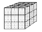
Rubik's cube is a simple looking puzzle. It is a cube with nine tiles on each face. In its solved state each of the sides is made up of tiles of the same color, with a different color for each side. Each of the tiles is actually part of a small cube, or cubie. Each face of the cube (made up of nine cubies) can be rotated. The mechanical genius of the puzzle is that the same cubie can be rotated from multiple sides. A corner cubie can move with three sides, and edge cubie moves with two sides. Figure 12.1 shows a cube in the initial solved state, and after the right side was rotated 90 degrees clockwise.
Figure 12.1. A Rubik's Cube before and after the right side is rotated
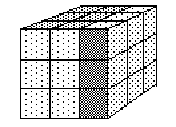
The problem is to take a cube whose sides have been randomly rotated and figure out how to get it back to the initial solved state. The scrambled cube might look like that of figure 12.2.
Figure12.2. A scrambled Rubik's Cube
The problem is, there are an astronomical number of possible ways to try to unscramble the cube, not very many of which lead to the solved state. To reach a solution using a blind search algorithm is not feasible, even on the largest machines. A human expert can unscramble the cube in well less than a minute.
The difficulty with solving the cube revolves around the fact that if you move one cubie, you have to move seven other cubies as well (the center one doesn't really go anywhere). This is not a big problem in the early stages of unscrambling the cube, but once a number of tiles are positioned correctly, new rotations tend to destroy the solved parts of the cube.
The experienced cube solver knows of complex sequences of moves which can be used to manipulate a small portion of the cube without disturbing the other portions of the cube. For example a 14 move sequence can be used to twist two corner pieces without disturbing any other pieces.
It is important to realize there are actually two different senses of solving the cube. One assumes the problem solver has no previous knowledge of the cube. The other assumes the individual is an expert familiar with all of the intricacies of the cube.
In the first case, the person solving the cube must be able to discover the need for complex sequences of moves and then discover the actual sequences. The program does not have anywhere near the level of "intelligence" necessary to solve the cube in this sense.
In the second case the person is armed with full knowledge of many complex sequences of moves which can be brought to bear on rearranging various parts of the cube. The problem here is to be able to quickly determine which sequences to apply given a particular scrambled cube. This is the type of "expertise" which is contained in the Rubik's cube program.
In the following sections we will look at how the cube is represented, what is done by searching, what is done with heuristics, how the heuristics are coded, how the cube is manipulated, and how it is displayed.
The core of the program has to be the knowledge representation of the cube and its fundamental rotations.
The cube lends itself to two obvious representation strategies. It can either be viewed simply as 54 tiles, or as 20 cubies (or pieces) each with either two or three tiles. Since much of the intelligence in the program is based on locating pieces and their positions on the cube, a representation which preserves the piece identity is preferred. However there are also brute force search predicates which need a representation which can be manipulated fast. For these predicates a simple flat structure of tiles is best.
The next decision is whether to use flat Prolog data structures (terms) with each tile represented as an argument of the term, or lists with each element a tile. Lists are much better for any predicates which might want to search for specific pieces, but they are slower to manipulate as a single entity. Data structures are more difficult to tear apart argument by argument, but are much more efficient to handle as a whole.
(The above statements are true for most Prologs which implement terms using fixed length records. Some Prologs however use lists internally thus changing the performance trade-offs mentioned above.)
Based on the conflicting design constraints of speed and accessibility, the program actually uses two different notations. One is designed for speed using flat data structures and tiles, the other is a list of cubies designed for use by the analysis predicates.
The cube is then represented by either the structure:
cube(X1, X2, X3, X4, .........., X53, X54)
where each X represents a tile, or by the list:
[p(X1), p(X2), ...p(X7, X8, X9), ...p(X31, X32), p(X33, X34), ...]
where each p(..) represents a piece. A piece might have one, two, or three arguments depending on whether or not it is a center piece, edge piece, or corner piece.
The tiles are each represented by an uppercase letter representing the side of the cube the tile should reside on. These are front, back, top, bottom, right, and left. (The display routine maps the sides to colors.) Quotes are used to indicate the tiles are constants, not variables. Using the constants, the solved state (or goal state of the program) is stored as the Prolog fact goalstate/1 :
goalstate( cube('F', 'R', 'U', 'B', ............)).
The ordering of the tiles is not important as long as it is used consistently. The particular ordering chosen starts with the center tiles and then works systematically through the various cubies.
Having decided on two representations, it is necessary to quickly change from one to the other. Unification has exactly the power we need to easily transform between one notation of the cube and the other. A predicate pieces takes the flat structure and converts it to a list, or visa versa.
pieces( cube(X1, X2, ....... X54), [p(X1), ......p(X7, X8, X9), .....]).
If Z is a variable containing a cube in structure notation, then the query
?- pieces(Z, Y).
Will bind the variable Y to the same cube in list notation. It can also be used the other way.
The following query can be used to get the goal state in list notation in the variable PieceState:
?- goalstate(FlatState),
pieces(FlatState, PieceState).
FlatState = cube('F', 'R', 'U', 'B', ......).
PieceState = [p('F'), p('R'), ....p('R', 'U'),
....p('B', 'R', 'F'), ....].
The first goal unifies FlatState with the initial cube we saw earlier. pieces/2 is then used to generate PieceState from FlatState.
Unification also gives us the most efficient way to rotate a cube. Each rotation is represented by a predicate which maps one arrangement of tiles, to another. The first argument is the name of the rotation, while the second and third arguments represent a clockwise turn of the side. For example, the rotation of the upper side is represented by:
mov(u, cube(X1,
...X6, X7, X8, X9, ...),
cube(X1, ...X6, X20, X19, X21, ...))
We can apply this rotation to the top of the goal cube:
?- goalstate(State), mov(u, State, NewState).
The variable NewState would now have a solved cube with the upper side rotated clockwise.
Since these can be used in either direction, we can write a higher level predicate that will make either type of move based on a sign attached to the move.
move(+M, OldState,
NewState):-
mov(M, OldState, NewState).
move(-M, OldState,
NewState):-
mov(M, NewState, OldState).
Having now built the basic rotations, it is necessary to represent the complex sequences of moves necessary to unscramble the cube. In this case the list notation is the best way to go. For example, a sequence which rotates three corner pieces is represented by:
seq(tc3, [+r, -u, -l, +u, -r, -u, +l, +u]).
The sequence can be applied to a cube using a recursive list predicate, move_list/3:
move_list([], X, X).
move_list(
[Move|T], X, Z):-
move(Move, X, Y),
move_list(T, Y, Z).
At this point we have a very efficient representation of the cube and a means of rotating it. We next need to apply some expertise to the search for a solution.
The most obvious rule for solving Rubik's cube is to attack it one piece at a time. The placing of pieces in the solved cube is done in stages. In Black & Taylor's book they recognize six different stages which build the cube up from the left side to the right. Some examples of stages are: put the left side edge pieces in place, and put the right side corner pieces in place.
Each stage has from one to four pieces that need placement. One of the advantages of writing expert systems directly in a programming language such as Prolog, is that it is possible to structure the heuristics in an efficient, customized fashion. That is what is done in this program.
The particular knowledge necessary to solve each stage is stored in predicates, which are then used by another predicate, stage/1, to set up and solve each stage. Each stage has a plan of pieces it tries to solve for. These are stored in the predicate pln/2. It contains the stage number and a list of pieces. For example, stage 5 looks for the four edge pieces on the right side:
pln(5, [p('R', 'U'), p('F', 'R'), p('R', 'D'), p('B', 'R')]).
Each stage will also use a search routine which tries various combinations of rotations to position a particular target piece. Different rotations are useful for different stages, and these too are stored in predicates similar to pln/2. The predicate is cnd/2 which contains the candidate rotations for the stage.
For example, the first stage (left edge pieces) can be solved using just the simple rotations of the right, upper, and front faces. The last stage (right corner pieces) requires the use of powerful sequences which exchange and twist corner pieces without disturbing the rest of the cube. These have names such as corner-twister 3 and tri-corner 1. They are selected from Black and Taylor's book. These two examples are represented:
cnd(1, [r, u, f]).
cnd(6, [u, tc1, tc3, ct1, ct3]).
The stage/1 predicate drives each of the stages. It basically initializes the stage, and then calls a general purpose routine to improve the cube's state. The initialization of the stage includes setting up the data structures that hold the plan for the stage and the candidate moves. Stage also reorients the cube for the stage to take advantage of symmetries and/or make for better displays.
The stage/1 predicate calls the main working predicates which search for the rotations to put a given piece in place, and update all of the appropriate data structures. The representation of the partially solved cube is a key design issue for this portion of the program.
There are predicates in the program which search through a cube in list-piece notation (rather than tile notation) and determine where a piece is, or conversely, which piece is in a given position. These predicates are useful for many portions of the program but are too slow to be used for testing whether a given search has been successful or not. This is true since they not only have to check for the new piece being placed, but they would also have to insure that none of the previously placed pieces have moved.
Unification is again the answer. So far, there are two cube/54 terms used in the program. One represents the final solved state of the cube, and the other represents the current state of the cube. We introduce a third cube/54, referred to as the criteria, which is used to denote which tiles are currently in place, and the tiles of the cubie which is currently being positioned.
Initially all of the arguments of this third cube are variables. This structure will unify with any cube. As pieces are put in place, the variables representing tiles of the criteria cube are unified with the corresponding tiles of the solved cube. In this case, the criteria cube will only unify with a cube that has those corresponding tiles in place.
As the program attempts to place each piece, it binds another piece in the criteria. For example, as the program attempts to position the sixth piece, the improve/2 predicate first binds the sixth piece in the criteria with the solved state. At this point then, the first six pieces will have bound values the same as the solved state. The remaining tiles will be represented by unbound variables which unify with anything. The criteria cube will then successfully unify with any cube that has the first six pieces in place.
Now that we have a plan of attack on the cube, and a means of representing the current state, and the criteria for testing if a given piece is in place, we can institute a very fast search routine. The core routine to the Rubik's cube program is a predicate rotate/3. It is called:
rotate(Moves, State, Crit).
The variable Moves is unbound at calling, and contains the list of moves necessary to position the piece after the search has succeeded. State is the current state of the cube, and Crit is the criteria for this stage of the solution. Crit has all of the pieces found so far bound, as well as the one additional piece for this search. rotate/3 searches for a sequence of moves which will put the new piece in place without disturbing the existing pieces.
The rotate/3 predicate illustrates the tremendous power and compactness of Prolog code. At the same time it illustrates the difficulty of understanding some Prolog code. Prolog's power derives from the built in backtracking execution and unification. Both of these features help to eliminate many of the standard programming structures normally used. Thus, a predicate like rotate/3 has a fraction of the code it would take in another language (and executes fast as well), but it requires a good understanding of the underlying execution behavior of Prolog to understand it.
rotate([], State, State).
rotate(Moves,
State, Crit):-
rotate(PriorMoves, State, NextState),
get_move(ThisMove, NextState, Crit),
append(PriorMoves, [ThisMove], Moves).
The rotate/3 predicate does a breadth first search as can be seen by the fact that it calls itself recursively before it calls the move generation predicate get_move/3. Since the application of moves and testing is so fast, and the depth of search is never great, intermediate results are not saved as in a normal breadth first search. Instead, they are just recalculated each time.
The append/3 predicate can be used to build lists. In this case it takes ThisMove and appends it to the end of the list PriorMoves, generating a new list, Moves.
The candidate moves for a given stage are stored in a predicate cand/1 (the actual program is a little more complex) which is maintained by the stage/1 predicate. For stage one, it would look like:
cand(r).
cand(u).
cand(f).
The get_move/3 predicate is called with Move unbound, and the second and third arguments bound to the current state and criteria respectively. If the call to move/3 fails (because it does not rotate the cube into a position which unifies with the criteria), then cand/1 backtracks generating another possible move. When all of the positive moves fail, then get_move/3 tries again with negative moves.
get_move(+Move,
State, Crit):-
cand(Move),
mov(Move, State, Crit).
get_move(-Move,
State, Crit):-
cand(Move),
mov(Move, Crit, State).
The efficiencies in rotate/3 show the rational behind the early design decisions of cube representation. The get_move/3 predicate is called with State and Crit. If it generates a move which unifies with Crit, it succeeds, otherwise it fails and backtracks. All of this testing and analysis is done automatically by Prolog's pattern matching call mechanism (unification).
The entire logic of the breadth first search also happens automatically due to the backtracking behavior of Prolog. If get_move fails to find a move which reaches the criteria, rotate/3 backtracks into the recursive call to rotate/3. Since the recursive call to rotate/3 uses NextState as the criteria, and NextState is unbound, the recursive call will succeed in generating PriorMoves and a modified state. Now get_move/3 tries again with this new state to see if a single move will reach the criteria. This process repeats through as many levels of depth as is necessary to find a sequence of moves which reach the criteria.
In practice, any more than a three deep search begins to get tedious. The design of the program is such, that it does not require more than a three deep search to find and position any given piece.
The program as described so far almost works. However it turns out there are a few situations that will cause the search routines to dig too deep for a solution. These situations drastically affect the performance.
It was necessary to add more intelligence to the program to recognize situations that will not be easily unscrambled by the search routine, and to correct them before calling rotate/3.
One of the problems occurs when positioning pieces on the left side. If the piece to be positioned is currently on the right side, then a few simple moves will put it in place on the left side. However, if the piece is already on the left side, but in the wrong position, then it will have to be moved to the right and back to the left. This longer sequence of moves takes longer to search for, so one of the extra heuristics looks for this situation.
The heuristics analyze the cube, test for this condition, and blindly move the piece to the right if it occurs. Then the normal search routine gets it back into its proper place. There are a couple of situations like this which are covered by the heuristics.
It is tempting to think of adding more and more of these heuristics to straighten out the cube with less searching. There is a trade-off however, and that is it takes time to apply the heuristics, and the search routine is relatively fast. So a heuristic is only worthwhile when the search is slow. The program may be improved by additional heuristics, but the search will still be the core of the program.
A graphical representation of the cube is used to display the progress of the program. A window is kept for recording all of the moves used so far.
In addition the program contains a cube editor that allows you to describe that scrambled cube that has been on your shelf all these years. Just carefully apply the moves step by step and you will get it back to its original state.
I don't mind saying that I was pretty proud of myself for writing this program. It was one of my better hacks. At the time, I had a neighbor who was 12 years old and who had just gotten a computer. He loved it and used to come over to my house to hang out with someone who actually got paid for playing with these things.
I had finished an early version of the cube program and decided to knock his socks off. I said, look at this and ran the program. On my PC-XT it solved a randomly scrambled cube in about three minutes. I looked at him and waited for his awed response. There was nothing. I asked him what he thought. He said he wasn't impressed. His best time was 45 seconds.
12.1 - Improve the speed of the program by experimenting with more heuristics and more canned move sequences. Try to find the optimal balance between the powerful heuristics and sequences and the time it takes to search for them.
12.2 - Experiment with a version of the cube program which when given the goal of replacing two pieces without disturbing the others, can "discover" a sequence and remember it for future use.
Copyright ©1989,2000 Amzi! inc. All Rights Reserved.